Topic outline

  • General

    Welcome to the home page of the Introduction to Data Science Course. The course consists of short chapters that we will cover in each lecture. Before each lesson, please review the reading material and the videos. We will discuss the reading material in detail during the lesson. The lesson will finish with homework, where you will complete the quiz. To complete the quiz, you will most often need to do a small project, where you will analyze a dataset and answer the quiz's questions with the results of your analysis.

    This course is offered in the xAIM's master's program. The course is co-financed by the European Commission instrument "Connecting Europe Facility (CEF) Telecom" through the project "eXplainable Artificial Intelligence in healthcare Management project" (2020-EU-IA-0098), grant agreement number INEA/CEF/ICT/A2020/ 2276680.

    eu-xaim

    Copyright

    This material is offered under a Creative Commons CC BY-NC-ND 4.0 license.

    Software

    • Orange Data Mining, visit this webpage to install Orange and check out its documentation

    Additional Material and Communication Channels

    Dates and Online Sessions

    • Friday, March 3 (exploratory data analysis, clustering, cluster explanation)
    • Thursday, March 16 (dimensionality reduction, PCA and understanding of components, embedding and explanation of clusters)
    • Thursday, March 30 (classification, explanation with nomograms and other tricks)
    • Thursday, April 13 (regression, explanation with SHAP values)

    • Wednesday, June 7 (exam)

    All online sessions will be on Zoom and will start at 18:00 CET. We will finish before 20:30.

    Grading

    • 70% Four homework assignments, one after online session
    • 30% Exam, about 20 choice questions, lasting 1.5 hour
  • Workflows and Exploratory Data Analysis

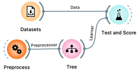
    We will start this course by exploring two data sets: a yeast gene expression data set and the socio-economic indices of world countries. We will learn that even with a few basic approaches, like sorting the data and visualizing the data in a scatterplot, we can already get some insight into the data patterns. This first lesson is also about learning the tool's mechanics, Orange, which we will use throughout the course.

    workflow-image

    Videos

    Lecture Notes

  • Hierarchical Clustering

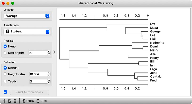
    Cluster detection is one of the basic procedures we use to analyze data. We can discover groups of users according to their user profiles through service usage, shopping baskets, behavior patterns, social network contacts, consumption of medicines, or hospital visits. We can cluster things according to their user interest profiles or semantic similarities. And we can find groups of documents according to text, keywords, user interest, and ratings. We can cluster anything else, provided we can measure the similarity between the entities we would like to group. Among the many algorithms used today to detect clusters in data, the most well-known is the hierarchical clustering algorithm. It is, therefore, convenient to start the course with this algorithm.

    hierarchical clustering and dendrogram

    Videos

    Lecture Notes

    • Hierarchical clustering, including chapters on estimation of distances between data instances, estimation of distances between clusters, construction of hierarchical clustering, presentation of hierarchical clustering with a dendrogram, and how everything works in higher dimensions.
    • Explaining Clusters

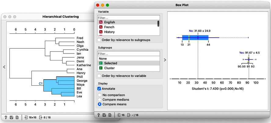
      Finding clusters in the data is one of the core approaches in exploratory data analysis and unsupervised data mining. We have already learned about a particular cluster-finding algorithm called hierarchical clustering. But even with a simple and small data set with student grades, we encountered a problem of cluster understanding. After obtaining the groups in the data, how can we explain what they are? How are the retrieved groups different from the rest of the data? Are these differences intuitive, and can they provide the grounds for explaining the results of the clustering? This lesson will re-use the Box Plot widget and show how to construct simple workflows for cluster explanation. Namely, we can use Box Plot to subset the data by cluster membership and provide a list of features sorted by how well they characterize the clusters. We claim that a set of characteristic features can provide the means for cluster explanation. While this explanation is not structured and does not include any feature interaction, it is a good start.

      explaining clusters

      Videos

      Lecture Notes

      • Explaining Clusters includes chapter on explaining clusters with ranking of most informative features and explaining clusters of countries that can be mapped on a geo map.
      • Outlier Detection, Silhouette Score and k-Means Clustering

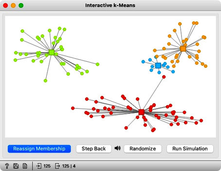
        This lecture focuses on the k-means clustering algorithm. However, before diving into its mechanics, we need to understand the concepts of inliers and outliers. Specifically, given a clustering, how do we determine which data instances are most and least representative of the cluster? We will define a silhouette score that measures the representativeness of a data instance in a cluster. We will also show that the average silhouette score can be a good measure of clustering quality. In addition, we will introduce k-means, a faster alternative to hierarchical clustering that requires the user to set a parameter k - the desired number of clusters. We will demonstrate how an algorithm can determine the optimal value of k by testing different values and selecting the one with the highest average silhouette score.

        explaining clusters

        Videos

        Lecture Notes

        • k-Means Clustering includes chapters on k-means and a demonstration on how to use k-means clustering and to explain clusters in the zoo data set.
        • Homework 1

          In this assignment, you will construct the data set and use techniques that we have learned so far to analyze it and gain insight into data set's patterns and clusters.

        • Dimensionality Reduction with Principal Components Analysis

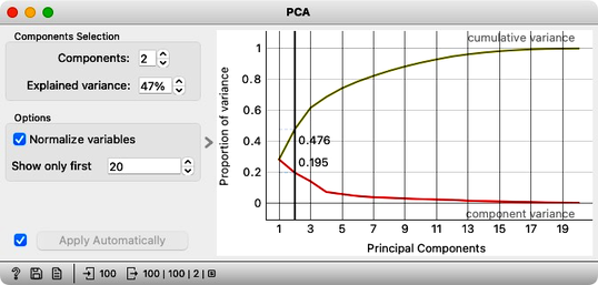
          While clustering is useful for identifying groups of similar data instances, it doesn't provide information about the similarity between individual data points or their distances. Visualizing data in a two-dimensional map can be a great way to gain insight into these relationships. However, to achieve this type of visualization, we must first reduce the data's dimensionality from its original feature space to two dimensions. In our lectures, we will introduce three different techniques for performing this dimensionality reduction, but only one involves finding a low-dimensional projection. This technique, called principal component analysis, identifies the projection that best captures the most spread-out parts of the data. When the resulting dimensionality is one or two, we can more easily understand the structure of the data.

          explaining clusters

          Videos

          Lecture Notes

          • Data embedding: MDS and t-SNE

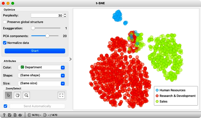
            There are two additional methods for reducing the dimensionality of data, namely MDS and t-SNE, which differ from PCA in that they do not project the data onto a lower-dimensional space. Instead, they optimize specific criteria functions to construct low-dimensional data representations. MDS seeks to minimize the pairwise difference between the distances of two data instances in the original and embedded space. In contrast, t-SNE focuses on preserving the local structure of the data instances. Both MDS and t-SNE are embedding techniques. It's worth noting that the embeddings produced by MDS and the projections generated by PCA can be pretty similar. However, t-SNE can yield markedly different results for larger datasets, highlighting the importance of considering multiple methods for dimensionality reduction.

            explaining clusters

            Videos

            Lecture Notes

            • Homework 2

              In this assignment, you will use dimensionality reduction techniques and try to explain the clusters you will find in the resulting data maps.

            • Introduction to Classification, Overfitting, and Evaluation of Predictive Accuracy

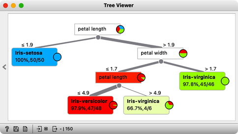
              Classification involves building a predictive model from data that's labeled with discrete class labels. To build such a model, we need a training dataset that includes both the independent variables (features) and dependent variable (class labels). The goal of classification is to develop a model that takes as input values of the independent variables and outputs the corresponding class label. The resulting model is then used to predict the class labels of new, unseen data based on their independent variables.

              In this lecture, we introduce one of the simplest classification models, known as a classification tree. However, we emphasize the importance of assessing the accuracy of the model on an independent test set. This ensures that the model is not overfitting to the training data and can generalize well to new data.

              classification tree

              Lecture Notes

              • Introduction to Classification includes an example of data for development of the classification model, introduction to classification trees, example of overfitting and motivation why we should always evaluate predictive accuracy on a separate test set
              • Classifiers

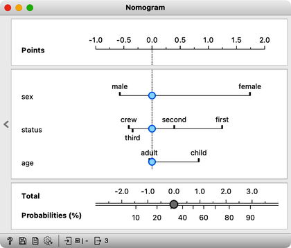
                In the past fifty years, machine learning researchers have developed an abundance of classifiers and their variants. All machine learning models aim to identify patterns in data, but they use different approaches to describe those patterns. For instance, decision trees divide the attribute space into hypercubes, while logistic regression identifies a hyperplane that separates the two classes. Support vector machines can discover more intricate decision boundaries depending on the kernel function employed. Naive Bayes classifiers are equivalent to logistic regression under the assumption of feature independence given a class, but its parameters are determined directly from the data, rather than via optimization. If accuracy is the primary concern and interpretability is of little consequence, core models can be combined, as in random forests. Rather than attempting to learn every technique, it is more important to thoroughly understand a few representative ones. This includes how to optimize their parameters to maximize accuracy and, if possible, how to explain the resulting model.

                nomogram

                Videos

                Lecture Notes

                • Classifiers overviews some core classifiers that used in machine learning. They have different modeling biases and offer different means of explaining the patterns in the data
                • Homework 3

                  In this assignment, you will reason about classification boundaries for different types of classifiers.

                • Feature Subset Selection

                  Intuitively, we might think that machine learning models should only be developed using features that have the strongest correlation with the class. However, we need to exercise caution when combining feature selection with accuracy estimation. One common, yet simple mistake is to first perform feature selection and then cross-validate the classifier on the reduced dataset. In this lesson, we will explain why this can result in overly optimistic outcomes and how to accurately evaluate the model.

                  nomogram

                  Lecture Notes

                  • Feature subset selection looks into techniques for feature ranking and feature selection, and explains how to correctly perform model evaluation that includes feature selection
                  • Scoring of Classification Models

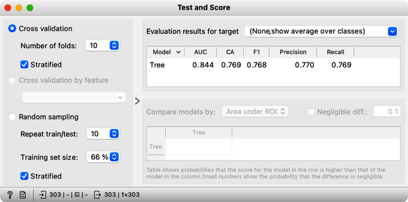
                    Here, we will briefly review various methods for estimating classifier accuracy, with the main point being that classification accuracy is affected by the distribution of classes and that other measures should be utilized to accurately assess predictive performance.

                    nomogram

                    Videos

                    Lecture Notes

                    • Working with Unstructured Data

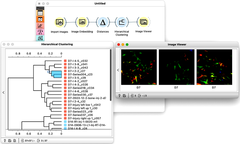
                      With unstructured data, we primarily mean images and text. We will focus on images but may also mention text and text mining during the lectures. Essentially, we need to represent such objects in a vector space. Once we have such representation, we can use any machine learning algorithm to find clusters and outliers and develop predictive models. To represent these objects with vectors, we will use already-developed deep models for images and text.

                      image-analytics

                      Lecture Notes

                      • Image Analytics considers images and shows how to embed them into vector space

                      Additional Reading

                      Videos

                      • Homework 4

                        In this homework we will use everything we have learned so far and apply it to image analytics.